four_methods_degs_union_combined_features <- read_csv("../test_TransProR/four_methods_degs_union_combined_features.csv")Rows: 1020 Columns: 1
── Column specification ────────────────────────────────────────────────────────
Delimiter: ","
chr (1): Feature
ℹ Use `spec()` to retrieve the full column specification for this data.
ℹ Specify the column types or set `show_col_types = FALSE` to quiet this message.all_degs_count_exp_gene_feature_auc_mapping_0_5_0_9 <- read_csv("../test_TransProR/all_degs_count_exp_gene_feature_auc_mapping_0.5_0.9.csv")Rows: 809 Columns: 3
── Column specification ────────────────────────────────────────────────────────
Delimiter: ","
chr (1): Gene
dbl (2): Feature, AUC
ℹ Use `spec()` to retrieve the full column specification for this data.
ℹ Specify the column types or set `show_col_types = FALSE` to quiet this message.all_degs_count_exp_gene_feature_auc_mapping_0_9 <- read_csv("../test_TransProR/all_degs_count_exp_gene_feature_auc_mapping_0.9.csv")Rows: 1421 Columns: 3
── Column specification ────────────────────────────────────────────────────────
Delimiter: ","
chr (1): Gene
dbl (2): Feature, AUC
ℹ Use `spec()` to retrieve the full column specification for this data.
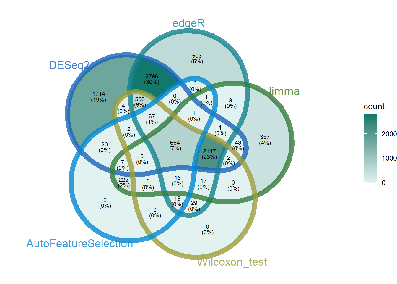
ℹ Specify the column types or set `show_col_types = FALSE` to quiet this message.AutoFeatureSelection<- four_methods_degs_union_combined_features$Feature
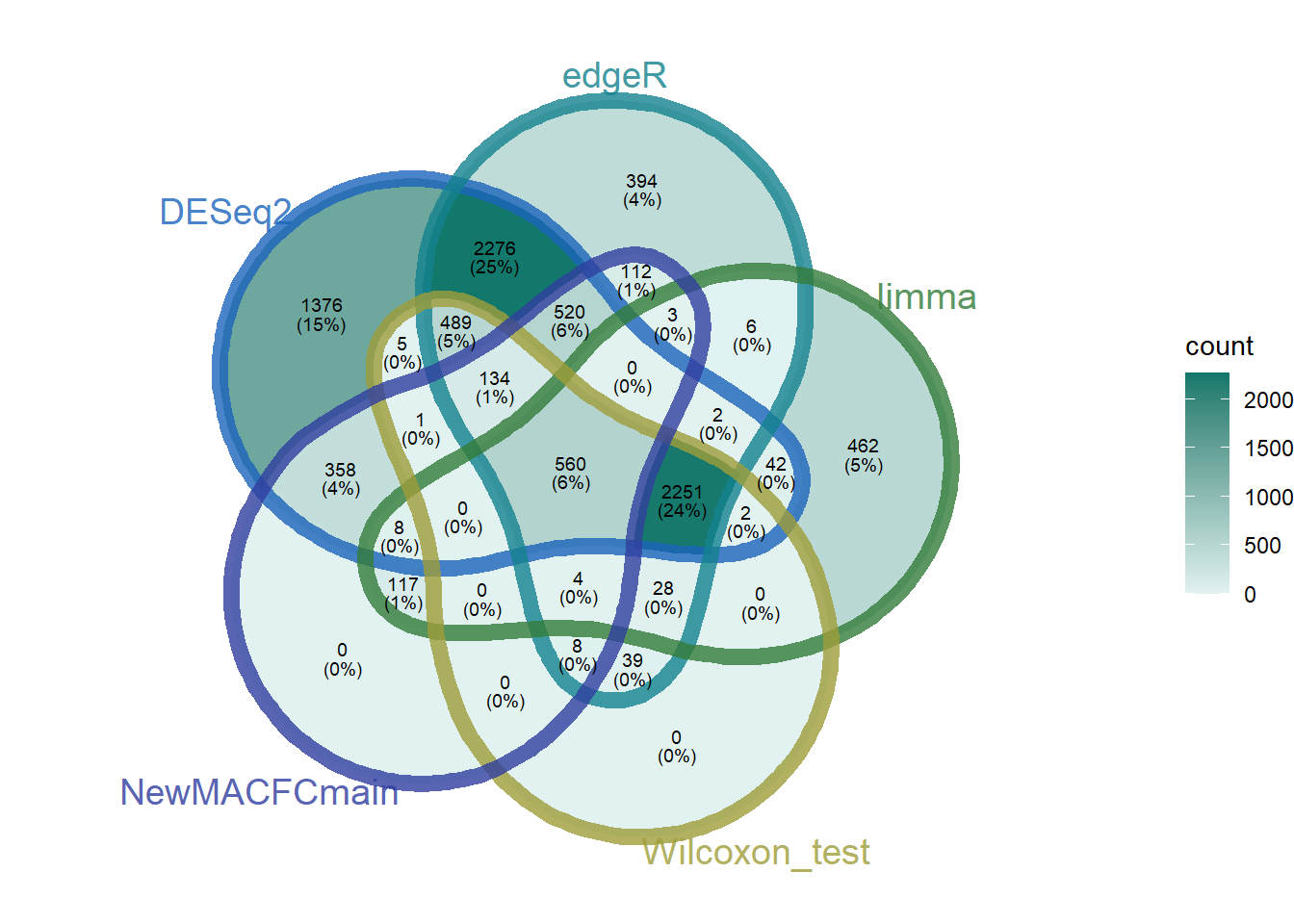
NewMACFCmain_0_5_0_9<- all_degs_count_exp_gene_feature_auc_mapping_0_5_0_9$Gene
NewMACFCmain_0_9<- all_degs_count_exp_gene_feature_auc_mapping_0_9$Gene
NewMACFCmain <- c(NewMACFCmain_0_5_0_9, NewMACFCmain_0_9)
DEG_deseq2 <- readRDS("../test_TransProR/Select DEGs/DEG_deseq2.Rdata")
DEG_edgeR <- readRDS("../test_TransProR/Select DEGs/DEG_edgeR.Rdata")
DEG_limma_voom <- readRDS("../test_TransProR/Select DEGs/DEG_limma_voom.Rdata")
outRst <- readRDS("../test_TransProR/Select DEGs/Wilcoxon_rank_sum_testoutRst.Rdata")